“Fropas”

One of the most exciting weather phenomena is the passage of a front, called a “Fropas” (FROH-pah) by meteorologists. Especially a strong cold front. A front is simply the boundary between a large mass of cold air and a large mass of warm air. When the cold air mass is moving in to replace the warm air, the front is called a “cold front.” Norwegian meteorologists used the name “front” to describe this boundary because the turbulent weather that occurs there reminded them of the battle fronts in World War I. One really nice thing about fronts is that you can often see them from space, and from radars. You can also see how the cloud patterns change as the front passes. I show some examples below for some fronts that passed through Boulder this spring.

From a satellite, cold fronts are sometimes quite easy to identify at least roughly. Here is the satellite image of a front that passed through Boulder on 12 May 2008. The image is centered on Colorado. The arc-shaped group of clouds, open to the northeast, marks the front.

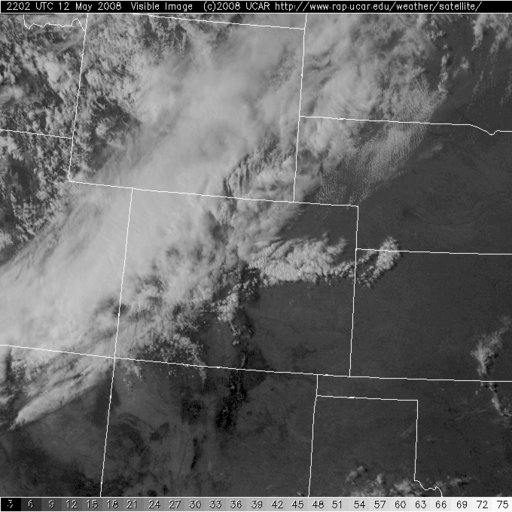
Figure 1. Satellite image close to time that a cold front passed through Boulder, Colorado, at 2202 UTC (16:02 or 4:02 p.m. Local Daylight Time) 12 May 2008, from http://www.rap.ucar.edu/weather/satellite/. The arc of clouds over northeastern Colorado marks the leading edge of the front. Colorado is the rectangular-shaped state in the middle of the figure. The northwest-southeast band that covers much of the northwest part of the image is related to the larger-scale pressure pattern higher up.

Note that all the charts and images (except for the cloud pictures) are from the UCAR weather page.

You can also see the arc of clouds in the center of Figure 2 (light bluish-green echoes). This means that the clouds contain some rain-sized particles. Behind (northeast) of the front, the weak signal is probably from insects. The blue-and-green echoes at the top of the radar image represent an area of precipitation.

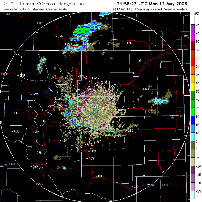
Figure 2. Radar image for 21:58 UTC (15:58 or 3:58 p.m. Local Daylight Time) showing the clouds (greenish-blue arc open to the northeast) corresponding to the cold front. The thick straight white lines show the north and east borders of Colorado; the circle is centered at the radar, at a distance of 150 km (slightly less than 100 miles). The thin white lines are the boundaries of the counties. From http://www.rap.ucar.edu/weather/radar/

Figure 3. Surface data at 00:45 UTC 13 May (18:45 or 6:45 p.m. Local Daylight Time 12 May). The circles (or squares) lie on the observation locations; the line from the circle/square points to the direction from which the wind is blowing; the number of barbs on the line gives the wind speed. Each full barb represents about 5 meters per second (10 knots), so two barbs mean about 10 meters per second, and three barbs mean about 15 meters per second. The front in this figure is slightly to the south of where it was in Figures 1 and 2. From

Figure 3 shows the wind direction and temperature changes across the front. Notice how the wind changes abruptly in eastern Colorado. In northeast Colorado, the winds are out of the northeast or the north-northeast, at around 20-30 knots (10-15 meters per second). In southeastern Colorado (ahead of the front), the winds are out of the southwest at 15 to 25 knots (7-12 meters per second). The temperatures (red numbers, Fahrenheit degrees) are warmer south of the front, where the wind is out of the southwest. (Note: we are just considering the airflow east of the mountains, which go north-south across the center of Colorado).

What does the front look like from a point?

When the front passed Boulder, the wind changed from west-southwest (270 to 225 degrees) to northeast (around 45 degrees, Figure 4). From both this figure and the map showing the winds, we see that the winds are coming together at the location of the arc. This means that the air has to go up at the arc. In fact, the warmer, lighter air flows up over the heavier, cold air. As the air rises, it cools, and water starts to condense, forming the clouds we see in the radar and satellite images.

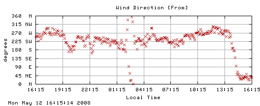
Figure 4. Wind direction at NCAR Foothills Laboratory, Boulder, Colorado, USA. Note the direction change between 13:15 and 16:15 (1:15 p.m and 4:14 p.m.) Local Daylight Time (Add six hours to get Universal Coordinated Time, or UTC). (270 degrees = west wind; 0 or 360 degrees = north wind, 90 degrees = east wind, 180 degrees = south wind). To get UTC, add 6 hours to Local Daylight Time. From
http://www.rap.ucar.edu/weather; click on “Foothills” under “current conditions” on the right hand side of the page.

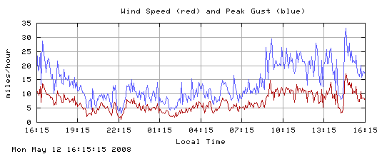
Figure 5. As for Figure 4, but for wind speed. Note the winds reached 20 miles per hour (~ 20 knots or 10 meters per second) and stronger near the front.

Once the wind shifted to northeast, it was bringing with it cooler air from the north, as shown in Figure 6. Notice that the cool air also has a higher dew point.

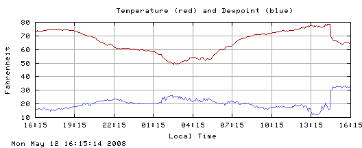
Figure 6. As for Figure 4, but for temperature (red) and dew point (blue). Note the sudden temperature drop at the same time the wind changes.

Have you heard the rule, “Air tends to move from high to low pressure.”? Figure 7 shows that air pressure was lowest around the time the front passed. So a map showing pressure would show the lowest pressures at or near the front’s (cloud arc’s) location.

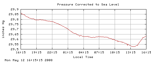
Figure 7. As in Figure 4, but for air pressure. Note the lowest pressure comes just before the sudden jump in temperature and dew point, and the sudden shift in wind direction. There are about 33.86 inches in one millibars (hectopascals).

I did not photograph the clouds on this day, but did for another frontal passage. The charts, shown below in Figure 8, show similar patterns to the three from the frontal passage on 12 May 2008, except that the winds behind the front were from the northwest (around 315 degrees).

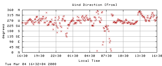
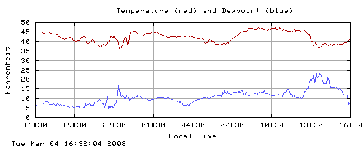
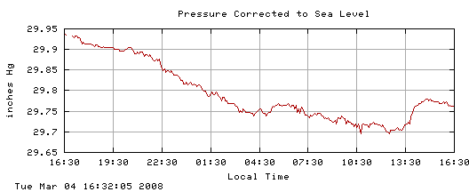
Figure 8. As in Figure 4, but for wind direction, temperature, and pressure, for frontal passage around 13:30 local time 4 March 2008, at NCAR Foothills Laboratory in Boulder, Colorado, USA. To get UTC, add 7 hours to local time (Local Standard Time).

Here are the clouds with this front. Note that the structure changed from spring-like fair-weather cumulus, to more wintry clouds, with some snow falling nearer the mountains.

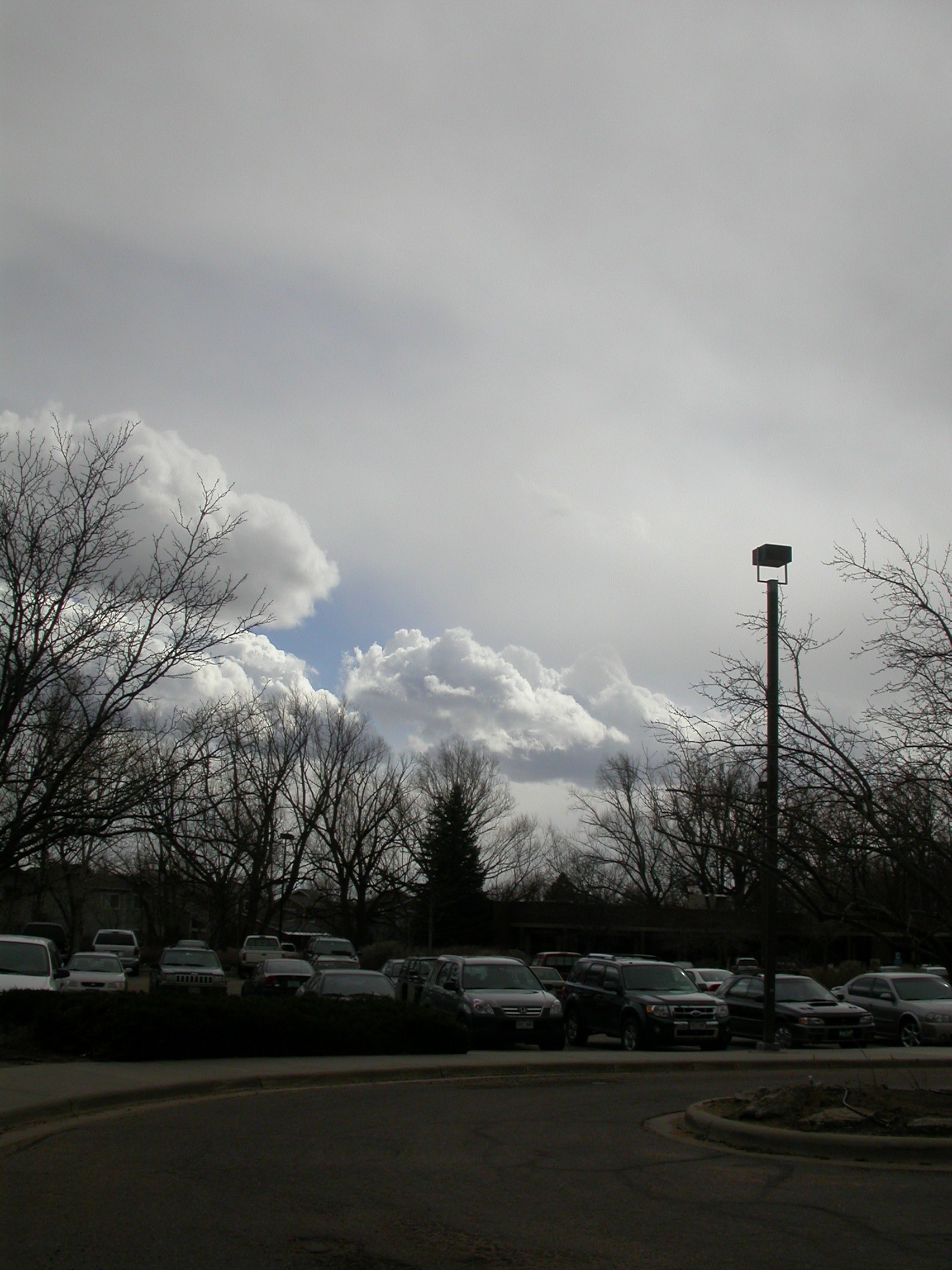
Figure 9. Looking south. Note the cumulus clouds to the south, and the less distinct clouds overhead at this time.

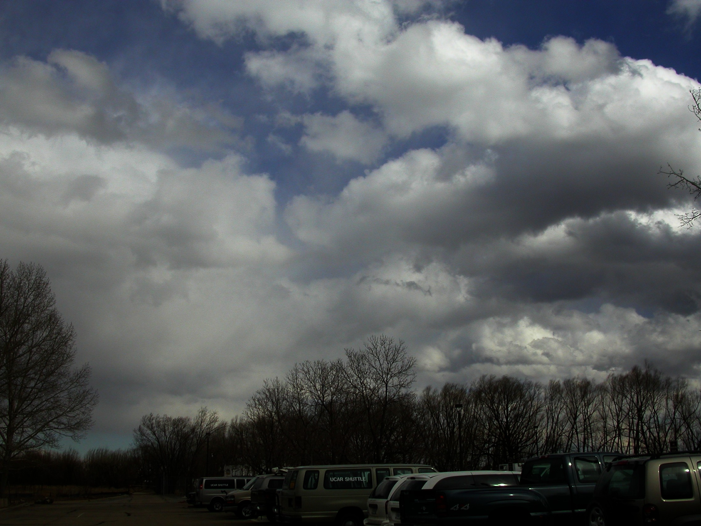
Figure 10. Looking east. Notice the change in structure from the right (southeast) to the left (northeast).

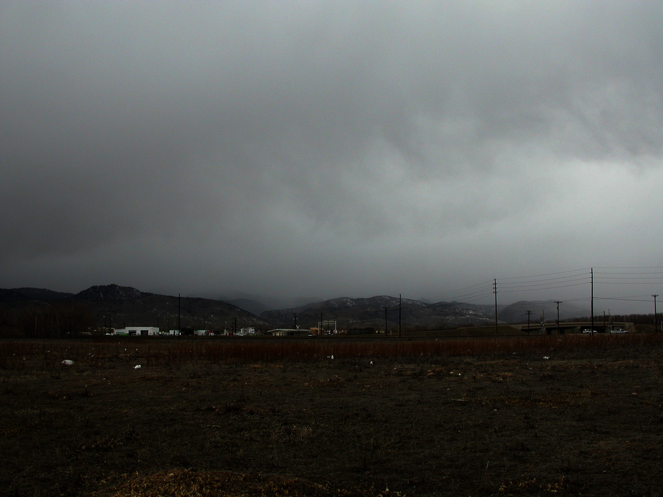
Figure 11. Looking northwest. Light snow is probably falling from the clouds.

When you see a front pass near your location, go to one of the satellite web sites mentioned in the 9 May 2008 blog, “Watching Clouds,” to see if the front can be seen from space. Or, if you are in one of the contiguous United States, you can go to http://www.rap.ucar.edu/weather, select “satellite” and click on your part of the country. You can also access the temperature maps (select “surface”) and radars (select “radar”) at this site.